
Probability density functions (PDFs) show how likely individual outcomes are for a random variable, while cumulative distribution functions (CDFs) add up these probabilities up to a specific point. PDFs help you understand the spread of data, and CDFs reveal the overall probability of falling within a certain range. Both tools are essential in statistics for estimating parameters, making predictions, and understanding data behavior. Exploring further will help you grasp how these functions support robust analysis and decision-making.
Key Takeaways
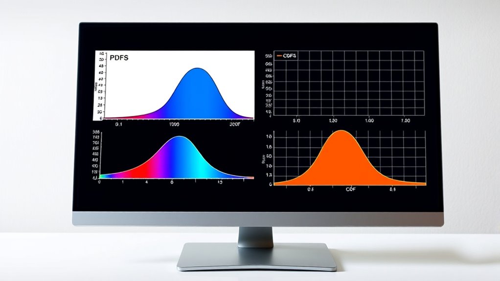
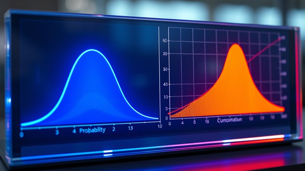
- PDFs depict the likelihood of a random variable taking specific values, illustrating data distribution.
- CDFs show the cumulative probability up to a certain point, aiding in understanding overall data behavior.
- PDFs are essential for parameter estimation and assessing how well models fit data.
- CDFs help determine probabilities of variables within ranges and compute confidence intervals.
- Both functions are fundamental in Bayesian inference, hypothesis testing, and statistical decision-making.
Probability density functions (PDFs) and cumulative distribution functions (CDFs) are fundamental tools in probability and statistics that help describe the behavior of random variables. When you’re working with data, these functions give you insights into the likelihood of different outcomes, enabling you to make informed decisions or predictions. PDFs show how probabilities are spread across possible values, while CDFs sum up these probabilities up to a certain point, providing a cumulative picture. Understanding both is essential for tasks like Bayesian inference and parameter estimation, where you need to update beliefs or find the most probable values based on observed data.
PDFs and CDFs are key tools for understanding data and updating beliefs in Bayesian analysis.
In Bayesian inference, PDFs are essential for expressing the likelihood of parameters given the data. You start with a prior distribution, which reflects your initial beliefs about the parameters before seeing any data. When new data arrives, you use the likelihood function—represented by the PDF—to update this prior. The result is a posterior distribution, which combines your prior knowledge with the evidence from the data. The CDF becomes useful here because it helps you determine the probability that the parameter falls within a certain range, making it easier to interpret your results. For example, if you want to find a 95% credible interval for a parameter, you can use the CDF to identify the bounds where the cumulative probability reaches 2.5% and 97.5%. This process is at the heart of Bayesian parameter estimation, allowing you to quantify uncertainty and make more precise inferences.
When estimating parameters, PDFs allow you to evaluate how well different values fit your data. By examining the shape of the likelihood function, you can identify the most probable parameter value—known as the maximum likelihood estimate—and assess the spread or uncertainty around it. The CDF further aids in this process by providing cumulative probabilities, which can be used to calculate confidence or credible intervals. These intervals convey the range within which the true parameter value likely resides, given your data and assumptions. Together, PDFs and CDFs give you an extensive framework to perform parameter estimation, especially in Bayesian contexts, where updating beliefs based on new evidence is central.
Ultimately, mastering PDFs and CDFs empowers you to analyze data more effectively. Whether you’re estimating parameters, testing hypotheses, or updating beliefs through Bayesian inference, these functions serve as foundational tools. They help you visualize, interpret, and communicate the uncertainty inherent in any statistical analysis, making your conclusions both robust and meaningful. By understanding their roles and how to leverage them, you strengthen your ability to work with random variables and extract valuable insights from data.
probability density function calculator
As an affiliate, we earn on qualifying purchases.
As an affiliate, we earn on qualifying purchases.
Frequently Asked Questions
How Do PDFS Differ From Probability Mass Functions?
You’ll find that probability density functions (pdfs) apply to continuous variables, representing the likelihood of a value within an interval, while probability mass functions (pmfs) work with discrete variables, giving exact probabilities for specific outcomes. The key difference is that pdfs don’t give direct probabilities but instead describe probability density, which you integrate over an interval, whereas pmfs assign probabilities directly, making their probability interpretation clearer for discrete cases.
Can a CDF Ever Decrease? Why or Why Not?
Think of a CDF as a rising tide; it can never decrease because it’s designed to always move upward or stay steady. It’s monotonically increasing, reflecting probability constraints that ensure the chance of an event happening by a certain point never drops. If it decreased, it would break these rules, making it impossible for the CDF to accurately represent cumulative probabilities. So, no, a CDF can’t ever decrease.
How Are PDFS Used in Real-World Data Analysis?
You use PDFs in real-world data analysis to model the likelihood of different outcomes, which helps in risk assessment and data modeling. For example, you might analyze financial returns or predict product failures. By understanding the shape of a PDF, you can identify high-risk areas or optimize processes. This application enables you to make informed decisions, minimize risks, and improve accuracy in predicting future events based on the data.
What Is the Relationship Between PDFS and Moments?
Moments measure the many, mirroring the map of distribution characteristics. You calculate moments by integrating the pdf with powers of the variable, revealing key insights like the mean and variance. These moments help you understand the shape and spread of data, connecting directly to distribution properties. fundamentally, the pdf fuels moments calculation, providing a foundation for deciphering the distribution’s details and defining its overall behavior.
How Do CDFS Help in Hypothesis Testing?
You use CDFs in hypothesis testing to determine the probability of observing a value as extreme or more extreme than your test statistic, which helps in threshold testing. By comparing this probability to your significance level, you interpret the p-value to decide whether to reject the null hypothesis. CDFs consequently provide a clear way to assess the strength of evidence against the null, guiding your decision-making process.
cumulative distribution function software
As an affiliate, we earn on qualifying purchases.
As an affiliate, we earn on qualifying purchases.
Conclusion
Understanding probability density functions and cumulative distribution functions is like having a map and compass for maneuvering randomness. They guide you through the peaks and valleys of probability, revealing where chances gather and how they accumulate. Mastering these tools lets you tame uncertainty, turning chaos into clarity. Think of them as your trusted lighthouse, illuminating the unknown waters of probability, so you can confidently steer your way through the unpredictable seas ahead.
Bayesian inference tools
As an affiliate, we earn on qualifying purchases.
As an affiliate, we earn on qualifying purchases.
statistical parameter estimation books
As an affiliate, we earn on qualifying purchases.
As an affiliate, we earn on qualifying purchases.