
Understanding the difference between discrete and continuous random variables is key to proper data analysis. Discrete variables take specific, separate values, like counting cars or students, and are described by probability mass functions (PMFs). Continuous variables, like height or temperature, can take any value within a range and are modeled with probability density functions (PDFs). Knowing which type you’re dealing with helps you select the right methods and interpret data accurately—your next step will clarify these concepts further.
Key Takeaways
- Discrete random variables take specific, countable values, while continuous variables can assume any value within a range.
- Discrete variables are described by a probability mass function (PMF); continuous variables use a probability density function (PDF).
- PMFs assign probabilities to individual outcomes; PDFs provide probabilities over intervals, with total area equal to 1.
- Recognizing variable type influences the choice of statistical methods and how data is modeled and interpreted.
- Discrete variables often involve counting, whereas continuous variables involve measurement and data clustering.

When studying probability and statistics, understanding the difference between discrete and continuous random variables is essential. These two types of variables form the foundation for analyzing data and predicting outcomes. Discrete random variables take on specific, separate values, like the number of cars passing a street or the number of students in a class. Continuous random variables, on the other hand, can take any value within a range, such as height, weight, or temperature. Recognizing this distinction helps you choose the right methods for modeling and analyzing data.
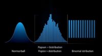
A key tool for understanding discrete random variables is the probability mass function (PMF). The PMF assigns probabilities to each individual value the variable can take. For example, if you’re counting the number of heads in a series of coin flips, the PMF tells you the likelihood of getting exactly zero, one, two, or more heads. The shape of the distribution in a discrete case is often represented by a bar graph, where each bar’s height shows the probability for that specific value. These distribution shapes can vary widely, from uniform distributions where every outcome is equally likely, to skewed or bimodal shapes depending on the scenario.
In contrast, continuous variables are described by probability density functions (PDFs), which differ from PMFs because they assign probabilities over ranges rather than specific points. The total area under the curve of a PDF always equals one, representing the certainty that the variable falls somewhere within the range. Unlike discrete distributions with distinct bars, the distribution shape of a continuous variable is smooth and can take various forms—bell-shaped for normal distributions, skewed, or uniform, depending on the data. Understanding the types of headphone jacks and their compatibility can be useful when selecting audio equipment for data analysis or multimedia presentations.
Understanding the distribution shapes of both types of variables helps you interpret data more effectively. For discrete variables, the shape can reveal if certain outcomes are more probable or if the data is evenly spread. With continuous variables, the shape of the PDF indicates where data tends to cluster or spread out. Recognizing these differences allows you to select appropriate statistical tools, such as calculating probabilities or making predictions. Whether working with counts or measurements, grasping whether your data is discrete or continuous guides your analysis and improves your ability to interpret real-world phenomena accurately.
Top picks for "random variabl discrete"
Open Amazon search results for this keyword.
As an affiliate, we earn on qualifying purchases.
Frequently Asked Questions
How Do I Choose Between Discrete and Continuous Models?
You should choose between discrete and continuous models based on your data collection methods and the nature of your data. If your data involves countable, separate values like the number of students, a discrete model with probability distributions suits best. If your data covers measurements that can take any value within a range, like height or temperature, a continuous model is more appropriate. Always match your model to the type of data you’re analyzing.
Can a Variable Be Both Discrete and Continuous?
A variable can be both discrete and continuous, creating mixed variable classifications that can complicate your analysis. This blending impacts measurements because some data points are countable, while others are fluid and infinite. When you encounter such a mixed variable, you need to carefully choose models that accommodate both aspects, ensuring your analysis remains accurate and meaningful. Recognize the remarkable reality that variables can be both, blending the best of both worlds.
What Are Common Examples of Mixed-Type Variables?
Mixed-type variables combine features of categorical and ordinal data, making them common in real-world scenarios. For example, a survey asking for your education level (high school, bachelor’s, master’s) and your satisfaction rating (poor to excellent) involves both categorical and ordinal data. You might also encounter variables like a product’s quality rating combined with its color, where the variable captures both categories and ordered preferences, illustrating mixed-type variables in everyday data analysis.
How Does Measurement Precision Affect Variable Classification?
Did you know that over 80% of scientists face measurement ambiguity in their data? Your measurement precision directly impacts variable classification—imprecise measurements can blur the line between discrete and continuous variables. When data resolution is low, it becomes harder to distinguish between the two, causing classification issues. Better measurement accuracy reduces data ambiguity, helping you classify variables correctly and make more reliable inferences.
Are There Real-World Scenarios Where Variables Change Type?
Yes, in real-world scenarios, variables can change type due to measurement accuracy. For instance, a temperature reading with low precision might be treated as continuous, but if measurement tools improve, it could be categorized as discrete. Your understanding of measurement accuracy influences variable categorization, as more precise measurements often convert variables from discrete to continuous. Recognizing these changes helps you interpret data accurately and adapt your analysis accordingly.
Conclusion
Understanding the difference between discrete and continuous random variables is like revealing the secrets of the universe—it’s truly mind-blowing! You now see how discrete variables jump from one value to another, while continuous variables flow seamlessly like a never-ending river. With this knowledge, you’re equipped to analyze real-world data more effectively. Explore data with confidence, knowing you’re armed with the most powerful tools in the universe—your newfound understanding of random variables!