The EM Algorithm Explained Step by Step

The EM algorithm helps you estimate model parameters when data is incomplete or has hidden parts. First, you start with an initial guess, then perform the E-step, where you calculate the expected value of hidden variables based on current parameters. Next, in the M-step, you maximize this expected likelihood to update your estimates. You keep repeating these steps until the estimates stabilize, making your model more accurate. Keep exploring to uncover more about how this powerful process works.

Key Takeaways

• The EM algorithm iteratively estimates parameters by alternating between the E-step (computing expected hidden variables) and the M-step (maximizing likelihood).
• Begins with an initial guess of model parameters, then refines estimates through repeated cycles.
• The E-step calculates expected sufficient statistics for hidden data based on current parameters.
• The M-step updates parameters to maximize the expected log-likelihood from the E-step.
• Continues iterations until parameter estimates stabilize, converging to the maximum likelihood solution.

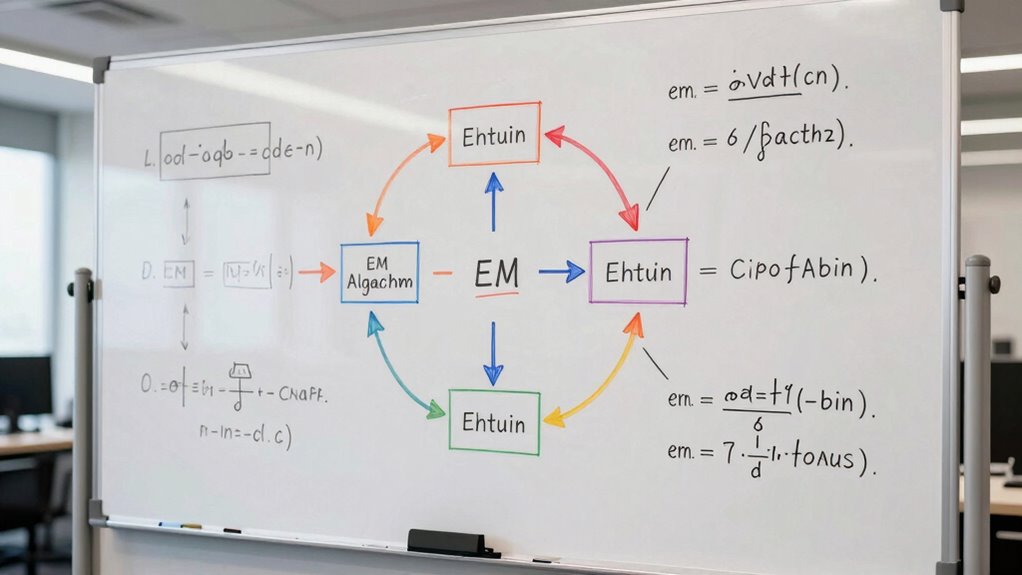
Ever wondered how statisticians estimate complex models with incomplete data? The answer often lies in the Expectation-Maximization (EM) algorithm, a powerful method used to find maximum likelihood estimates when some data points are hidden or missing. When you deal with real-world data, it’s common to encounter hidden variables—unobserved factors that influence your observations but aren’t directly measurable. These hidden variables make traditional estimation techniques tricky, but the EM algorithm offers a structured way to handle such challenges. It leverages Bayesian inference principles by treating the hidden variables as latent, and iteratively refines parameter estimates based on what’s observed and what’s unobserved.

The EM algorithm uses Bayesian principles to estimate models with hidden or missing data effectively.

The process starts with an initial guess of the model parameters. In the Expectation step (E-step), you calculate the expected value of the log-likelihood function, considering the current parameter estimates. Fundamentally, you estimate the distribution of the hidden variables given the observed data and current parameters. This step involves calculating the expected sufficient statistics for the hidden variables, which can be viewed as filling in the gaps or “imputing” the missing data. By doing this, you incorporate Bayesian inference concepts, updating your beliefs about the hidden variables based on the observed data and the current model. Additionally, the contrast ratio impacts how well the model distinguishes between different components, influencing the convergence of the algorithm. The effectiveness of the EM algorithm often depends on the quality of the initial parameter guesses and the nature of the hidden variables, which can affect convergence speed and accuracy. Moreover, understanding the natural variability in data can help optimize the initialization process and improve convergence. Recognizing the importance of model assumptions can also significantly impact the success of the EM algorithm in practice.

Next comes the Maximization step (M-step). Here, you maximize the expected log-likelihood obtained in the E-step with respect to the model parameters. This step updates your estimates, making them more aligned with the observed data and the inferred hidden variables. The process then loops back to the E-step, using the new parameters to re-estimate the distribution of hidden variables, and then again to the M-step to refine the parameters. With each iteration, your estimates become more accurate, converging towards the maximum likelihood solution even when parts of the data are missing or hidden.

The beauty of the EM algorithm lies in its ability to handle incomplete data efficiently. By iteratively applying Bayesian inference principles, it systematically reduces uncertainty about the hidden variables. Over successive iterations, the estimates stabilize, providing you with a reliable set of parameters for your complex model. Whether you’re working with mixture models, hidden Markov models, or other latent variable frameworks, the EM algorithm simplifies the estimation process in the presence of hidden variables, making it an essential tool in the statistician’s toolkit.

Frequently Asked Questions

How Does the EM Algorithm Compare to Other Optimization Methods?

You’ll find that the EM algorithm often offers good model convergence, especially with incomplete data, but it can be slower than methods like gradient descent. Its computational efficiency varies depending on the problem size and complexity. While it guarantees convergence to a local maximum, other optimization techniques might reach the global maximum faster. Overall, EM balances ease of implementation with reliable convergence, but it’s not always the fastest choice for optimization tasks.

Can the EM Algorithm Handle Missing or Incomplete Data Effectively?

The EM algorithm can handle missing data and incomplete datasets like a superhero saving the day. It estimates the missing values iteratively, filling in gaps with the best possible guesses, then refines those estimates until they converge. This process makes it especially effective for real-world problems where data is often incomplete or messy. So, yes, the EM algorithm is a powerful tool for managing missing or incomplete data efficiently.

What Are Common Challenges or Pitfalls When Implementing EM?

When implementing the EM algorithm, you often face challenges like convergence issues, where the algorithm stalls or oscillates, making it hard to reach a reliable solution. You also risk getting trapped in local optima, meaning your results might not be the best overall. To overcome these pitfalls, you should run multiple initializations, monitor convergence carefully, and consider alternative optimization strategies to improve your chances of finding the global maximum.

How Do You Choose Initial Parameters for the EM Algorithm?

You should select initial parameters carefully to enhance EM algorithm performance. Use domain knowledge, random initialization, or multiple runs with different starting points to find suitable initial parameter selection. This helps avoid local optima. Additionally, define clear convergence criteria, like a threshold for parameter change or likelihood improvement, to determine when the algorithm has sufficiently converged, ensuring reliable and efficient results.

What Are Practical Applications of the EM Algorithm Beyond Clustering?

Think of the EM algorithm as a detective solving mysteries beyond clustering. You use it in image reconstruction, natural language processing, and missing data imputation. By carefully selecting parameter initialization, you set the stage for smooth convergence, ensuring the algorithm doesn’t chase false leads. Its power lies in handling incomplete or complex data, making it invaluable across fields like bioinformatics, speech recognition, and finance—turning chaos into clarity.

Conclusion

And there you have it! Mastering the EM algorithm means you hold the secret weapon to unseal even the most complex data mysteries. With this step-by-step guide, you’ll navigate missing data like a superhero slicing through chaos with laser precision. Imagine transforming confusion into clarity faster than you can say “expectation-maximization”! So go ahead, conquer your data universe—because once you understand the EM algorithm, nothing can stop your analytical superpowers!