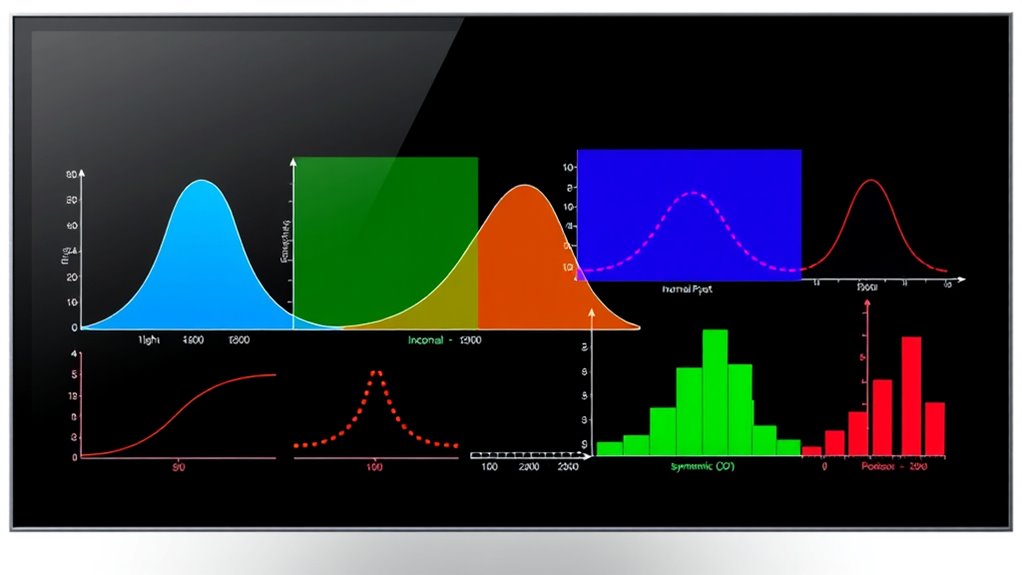

To master statistical analysis, you should know seven key probability distributions: Uniform, Binomial, Normal, Lognormal, Student’s T, Chi-Square, and F-distribution. These distributions help model different data types and support hypothesis testing. Each has unique characteristics, like shape and spread, influenced by specific parameters. Understanding these distributions is essential for accurate data interpretation. Stay with us to explore each distribution’s properties and applications in detail.
Key Takeaways
- The Beta, Gamma, and distributions involving degrees of freedom are fundamental for modeling diverse statistical phenomena.
- Common distributions include Uniform, Binomial, Normal, Lognormal, and Student’s T, each suited for specific data types.
- Distribution characteristics like mean, variance, skewness, and shape depend on parameters such as df1 and df2.
- These distributions are essential in hypothesis testing, determining critical values, and calculating p-values.
- Understanding these key distributions aids in accurate data modeling, inference, and decision-making across various fields.
Uniform Distribution

Have you ever wondered how to model situations where every outcome is equally likely? That’s where the uniform distribution comes in. It applies when all possible outcomes have the same chance of happening, whether the outcomes are discrete—like flipping a coin or rolling a die—or continuous, such as choosing a random number between 0 and 1. The refresh rate of projectors can also influence the overall viewing experience, especially during fast-paced gaming or action scenes. In electric bikes, the speed capabilities can vary widely, but within a uniform distribution, each speed within a specified range is equally probable. Graphically, a discrete uniform distribution appears as a flat line, while a continuous one is a rectangle. To find individual probabilities in discrete cases, you divide 1 by the total number of outcomes. For continuous cases, the probability density is constant across the interval.
Uniform distributions are symmetric, making the mean and median equal, which simplifies analysis in many real-world random events.
Binomial Distribution

Curious about how to model the number of successes in a fixed number of independent trials? The binomial distribution helps you do just that. It’s a discrete probability distribution that counts successes in a set number of trials, each with the same chance of success.
You need two parameters: the total number of trials (n) and the probability of success (p). Each trial results in success or failure, and the trials are independent. Understanding the divorce process in various states can help illustrate how outcomes depend on specific legal conditions and procedural steps. Additionally, the binomial distribution is often used in quality control scenarios to determine defect rates and reliability.
The distribution is used in real-world scenarios like coin tosses, quality control, or surveys. To calculate probabilities, you use the binomial formula involving combinations, success probability, and failures.
The mean is np, and the variance is np(1-p). It’s a practical way to analyze outcomes where two results are possible in multiple independent trials.
Normal Distribution
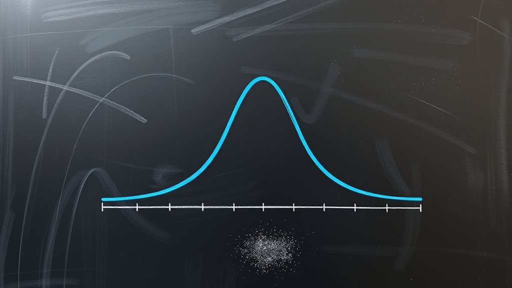
While the binomial distribution models discrete success counts in fixed trials, many real-world variables follow a continuous pattern. The normal distribution is the most common example, characterized by its symmetric, bell-shaped curve.
When graphed, it shows how data points tend to cluster around the mean, with fewer values appearing further away. Its key parameters are the mean (μ), which indicates the center, and the variance (σ²), which measures spread. The distribution’s probability density function describes how likely a value is within the range. The normal distribution’s properties make it a foundational concept in statistics, enabling researchers to make inferences about real-world data.
The mean, median, and mode are all equal, reinforcing its symmetry. Used extensively in statistics, science, and social sciences, the normal distribution helps analyze variables like test scores, measurement errors, and physical quantities that result from many independent factors. It is also fundamental in understanding glycolic acid product efficacy and other skincare trends in data analysis.
Lognormal Distribution
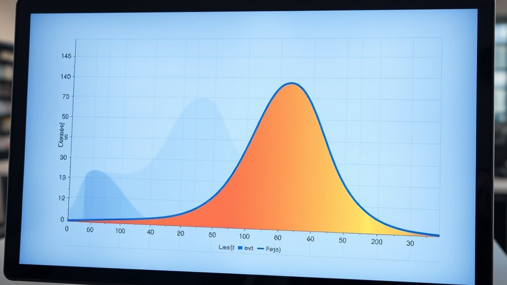
The lognormal distribution describes a continuous random variable whose logarithm follows a normal distribution. If ( Y = ln(X) ) is normally distributed, then ( X = e^Y ) is lognormally distributed, restricted to positive values. It is particularly useful in modeling Gold price movements, which often exhibit multiplicative effects and positive skewness. This distribution often models phenomena resulting from multiplicative processes, like incomes, stock prices, or biological measurements. It’s characterized by two parameters: (mu) (mean of (ln(X))) and (sigma) (standard deviation of (ln(X))). The probability density function (PDF) is (f_X(x) = frac{1}{xsigma sqrt{2pi}} expleft(-frac{(ln x – mu)^2}{2sigma^2}right)), and the cumulative distribution function (CDF) relates to the standard normal (Phi). It’s always positively skewed, with the median at (e^{mu}) and the mean at (e^{mu + sigma^2/2}). Understanding the distribution’s properties can aid in selecting appropriate models for real-world data exhibiting multiplicative effects.
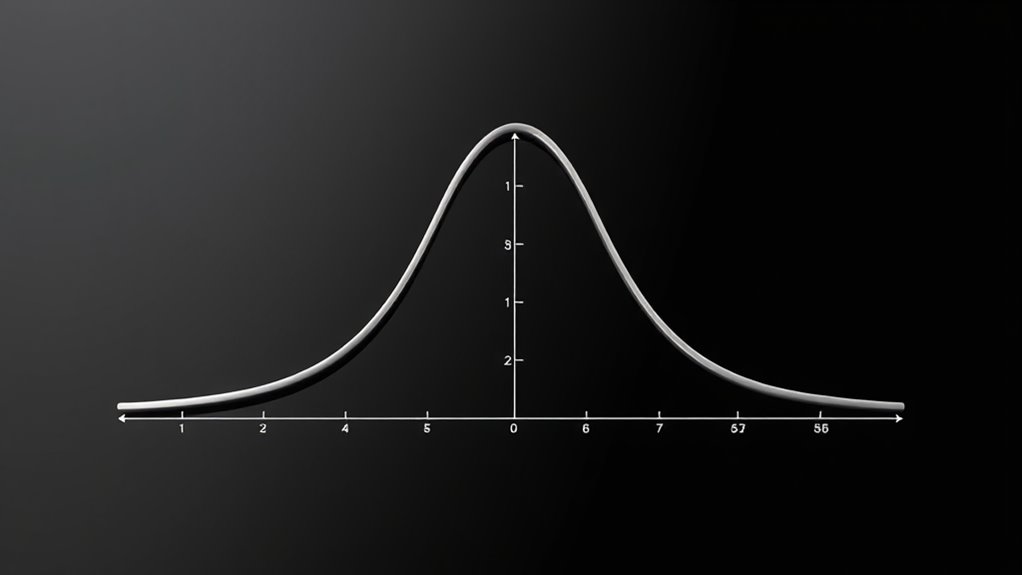
Student’s T-Distribution

The Student’s t-distribution is a symmetric, bell-shaped distribution similar to the normal distribution but with heavier tails, meaning it has a greater likelihood of producing extreme values. This makes it particularly useful when dealing with small sample sizes or unknown population variances. Its shape depends on degrees of freedom: fewer degrees lead to heavier tails, while larger degrees make it resemble the normal distribution more closely. The distribution’s mean is zero, and its variance exceeds one but approaches it as sample size increases. You’ll often use the t-distribution in hypothesis tests, confidence intervals, and estimating population parameters when the standard deviation isn’t known. Understanding the properties of probability distributions helps in selecting the appropriate model for data analysis. As your sample size grows, the t-distribution increasingly resembles the standard normal, making it versatile for different statistical scenarios. Recognizing the distribution’s shape is essential for accurate statistical inference.
Chi-Square Distribution

The chi-square (Χ²) distribution is a fundamental tool in statistical hypothesis testing, especially when evaluating variances and categorical data. It’s defined as the sum of squares of k independent standard normal variables, where k is the degrees of freedom.
The distribution is right-skewed, starting at zero and extending to infinity, with no negative values. Its shape depends on k; small k results in a highly skewed distribution, while larger k makes it more symmetric and closer to a normal shape. Understanding the distribution’s shape is crucial for selecting the appropriate tests and interpreting results accurately.
The mean equals k, and the variance is 2k. You often use the chi-square distribution in goodness-of-fit tests, tests of independence, and variance estimation. Attention to detail is crucial when applying this distribution to ensure accurate results.
Its key properties make it essential for analyzing categorical data and understanding the variability within data sets.
F-Distribution
Have you ever wondered how statisticians compare variances across different groups or populations? The F-distribution helps answer that question. It’s a probability distribution used in hypothesis testing, especially when comparing two variances from normal populations.
You’ll find it’s continuous and non-negative, defined as the ratio of two independent Chi-square distributions, each divided by its degrees of freedom (df1 and df2). The F-distribution plays a crucial role in analysis of variance (ANOVA), testing if group means differ considerably, and constructing confidence intervals for variance ratios. Additionally, understanding its probability density function helps in accurately calculating probabilities and critical values for hypothesis testing. Its application in hypothesis testing makes it an essential tool in statistical analysis.
Its probability density function involves the Beta and Gamma functions, depending on df1 and df2. Key statistics include the mean and variance, which are valid when df2 exceeds 2 and 4, respectively.
Frequently Asked Questions
How Do I Choose the Right Distribution for My Data?
When choosing the right distribution for your data, start by understanding if it’s discrete or continuous, and note any natural bounds.
Look at the data’s shape, symmetry, and peaks.
Use graphical methods and goodness-of-fit tests to compare different distributions.
Fit parameters with techniques like maximum likelihood, then validate your choice visually and statistically.
Keep it simple with standard distributions first, and refine as needed for accuracy.
What Are the Assumptions Behind Each Distribution?
Did you know that choosing the right distribution can make your analysis much more accurate?
When you examine assumptions, you see that normal distributions assume data is symmetric around the mean with a specific spread.
While uniform distributions require all outcomes to be equally likely.
Binomial models need fixed trials with independent binary outcomes.
And Poisson assumes events are rare and occur independently at a constant rate.
How Do Sample Size and Parameters Affect Distribution Shape?
You might wonder how sample size and parameters influence distribution shape.
As your sample size grows, sampling variability decreases, making the distribution more stable and closer to normal, thanks to the Central Limit Theorem.
Parameters like mean and standard deviation shape the distribution’s form and spread.
Larger samples tend to reduce skewness and better reflect the population, helping you make more accurate inferences and understand data behavior effectively.
Can These Distributions Be Used for Predictive Modeling?
You might find that these distributions are powerful tools for predictive modeling. For example, the Poisson distribution accurately predicts event counts, helping you forecast leads or customer visits.
The normal distribution, with its bell shape, models data like heights or errors.
The exponential distribution estimates waiting times between events.
Using these, you can improve your predictions and decision-making based on the nature of your data and the specific distribution’s strengths.
What Are Common Real-World Applications of Each Distribution?
You want to know how each distribution applies in real life. For binomial, think of predicting sports wins or customer choices.
Poisson helps in modeling traffic accidents or hospital outbreaks.
Uniform suits game development or lottery odds.
Normal distribution is key in IQ scores and stock markets.
Each distribution fits specific situations, so understanding their applications helps you analyze and predict outcomes more effectively in fields like finance, healthcare, and manufacturing.
Conclusion
Just as the universe follows certain laws, understanding these seven distributions equips you to navigate uncertainty with confidence. Like explorers charting unknown territories, mastering these concepts transforms complex data into meaningful insights. Whether you’re predicting outcomes or analyzing variability, these distributions are your compass. Embrace their stories, and you’ll discover a deeper grasp of probability’s vast landscape—turning the chaos of randomness into a map you can confidently follow.